The 15 Best Online Casinos in Australia for Real Money (2026)
Written by
 Ewan McAllister
Table of Contents
You can easily find a casino to take your money, but finding a site that’s actually worth your time and cash? That takes days, sometimes weeks, of digging.
It’s hard work, but someone has to do it. We evaluated over 150 online casinos available to Aussies against key ranking factors, from sign-up bonuses and mobile play to the quality of their game libraries.
After countless spins, tests, and some serious vetting, we’ve put together our definitive list of the best real money online casinos in Australia.
So, let’s take a look at the leading Aussie casino sites, their welcome offers, and a few standout aspects of each brand.
Toplist of the Best Australian Online Casinos

Up to $A4,000 + 350 Free Spins
Up to 20% cashback
Fortune Wheel bonuses
Instant 0% fee payouts


Up to A$2,500 + 250 Free Spins
Daily tournaments
Up to 13% weekly cashback
Crypto welcome bonus

Up to A$11,000 + 300 Free Spins
Progressive jackpot network
Over 500 live dealer games
Mobile app is available


Up to A$2,200 + 570 Free Spins
Variety of payment options
Daily casino bonuses
7,000+ games


Up to A$10,500 + 650 Free Spins
VIP program for all
Missions &Prize Drops
Huge welcome bonus

Up to A$6,000 + 250 Free Spins
High-roller bonus
Various pokie tournaments
Fast payment processing
Up to A$5,000 + 500 Free Spins
Low minimum deposit
Loyalty rewards for everyone
Wheel of Fortune
Up to A$2,000 + 100 Free Spins
20 no deposit free spins
10% live cashback offer
Special Lootbox promo

Up to A$8,000 + 400 Free Spins
Over 100 jackpot pokies
Fantastic live roulette collection
10% cashback for pokies

Up to A$5,000 + 300 Free Spins
Loyalty program
Progressive web app
Multiple reload promos

Up to A$5,000 + 300 Free
20% daily cashback
24/7 support
Active casino tournaments

Up to A$9,750 + 225 Free Spins
Great mobile casino
Top VIP Club
Crypto bonus for regulars

Up to A$1,500 + 300 Free Spins
5,000+ online pokies
Numerous FS bonuses
600+ live dealer games
Up to A$3,000 + 150 Free Spins
Tropical Fortune Lounge
Mobile-focused casino
Daily ‘Mystery Box’ promo
Up to A$4,500 + 350 FS + 1 Bonus Crab
8,000+ games
International live dealer tables
25% live cashback


Find the Best Real Money Casino Sites in Australia By Preference
You can start playing immediately with Stay Casino, which I have named the overall best online Australian casino, earning the highest marks across all parameters from all 15 listed casinos.
If you’re targeting a specific category of casinos based on preferences like fast payouts, top bonuses, or excellent mobile gaming, you should check out the top brands listed below.
#1 Stay Casino – Overall Best Casino for Australian Players in 2026
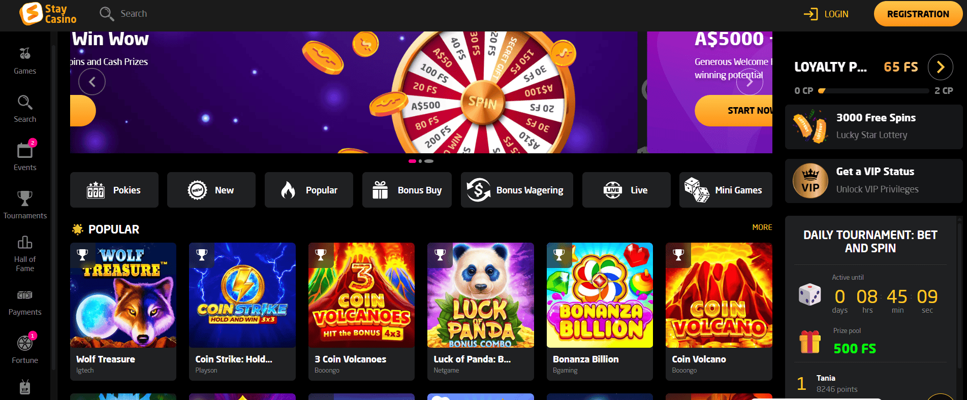
On the outside, Stay Casino seems like a run-of-the-mill online casino. However, when I started poking around and digging deeper into its operation, it came out as a top Australian online casino contender and ultimately beat the competition to take first place. Why? A ton of reasons.
I’ll start with the game lobby, which offers a diverse mix of pokies, jackpots, live and RNG card and table games like roulette, blackjack, poker, baccarat, and a collection of Mini Games.
Over roughly three weeks, I covered all game categories and played around 100 real money games, mostly pokies. Many of these games are budget-friendly, allowing for low-stakes gambling at A$1 or less, making it easy to have fun without overspending.
I also entered a daily pokie tournament for Pragmatic Play’s Drops and Wins pokies and managed to collect about 30 free spins over a few days. Keep in mind, participating in tournaments requires some patience and effort to earn rewards from the prize pools, but there’s no need to worry about spending too much since these tournaments have very few restrictions and are great for low-stakes players.
The Events calendar kept me in the loop about upcoming casino competitions throughout the week, which was quite helpful.
Bonuses and special promotions like the Fortune Wheel are sprinkled all around the site. I recommend reading the terms carefully before accepting any bonus offers. All bonuses come with a 40x wagering requirement, which is just a bit higher than what I usually prefer (30x-35x), and this might require a little extra effort to clear the bonus conditions.
When you’re ready to withdraw, I recommend Bitcoin or another familiar cryptocurrency. I used BNB to withdraw about A$3,800, and it took less than an hour for the casino to approve my request.
 Pros
Pros

 Cons
Cons

Fastest Payout Casino Sites in Australia
| Casino | Fastest Payment Method | Processing Time | Fees |
|---|---|---|---|
| Stay Casino | MiFinity | Up to 1 hour | None |
| SkyCrown | Litecoin | 5 - 15 minutes | None |
| CrownSlots | Bitcoin | 20 minutes | None |
The best online casinos in Australia must be ready to review and approve withdrawal requests quickly. Stay Casino, our top pick, offers fast withdrawals, with an average processing time of 24 hours or less. When I cashed out from the casino, it took about an hour for the operator to process my request via MiFinity.
I also selected SkyCrown as one of the fastest payout Aussie online casinos, where payouts with crypto are lightning-fast, often taking 2-5 minutes, and rarely exceeding 15 minutes when things go slowly.
CrownSlots is another crypto-friendly casino with ultra-fast withdrawal processing when using any crypto. I cashed out approximately A$2,800 using Bitcoin, and the entire process was completed in 20 minutes.
Top AU Mobile Casinos
| Casino | PWA | Mobile Bonus |
|---|---|---|
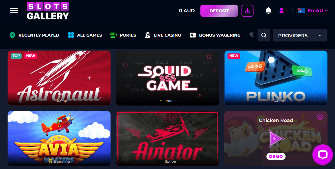
| Slots Gallery | Android & iOS | 25 - 125 FS every month |
| CrownSlots | Android & iOS | 30 - 110 FS every Thursday |
| DragonSlots | Android & iOS | 10 free spins for installing the PWA |
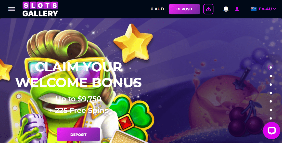
SlotsGallery is my first pick for mobile gambling. I have many reasons, but the most important one is that the casino is fast, has great bonuses (I love the monthly free spins), and it gives me access to all my favourite games.
CrownSlots is a close second, with a PWA app available, a long list of games, and this time, you’ll actually find regular mobile bonuses. So, why is it second? I’ve noticed a few times that if you’re playing for a long time, some games start to lag, and the battery dries faster.
DragonSlots also has a non-native web application that’s pretty good to use. I did notice a slightly better app performance on my iPhone compared to the Android-powered Samsung Galaxy I used, but the difference is minimal. When you install the app, DragonSlots will award 10 free spins.
Top Pokie Sites for Aussies
| Casino | Best Pokie to Play | Return to Player (RTP) |
|---|---|---|
| Wild Tokyo | Gates of Olympus 1000 | 96.5% |
| DragonSlots | Aztec Clusters | 97% |
| King Billy | Gold Rush With Johnny Cash | 96.14% |
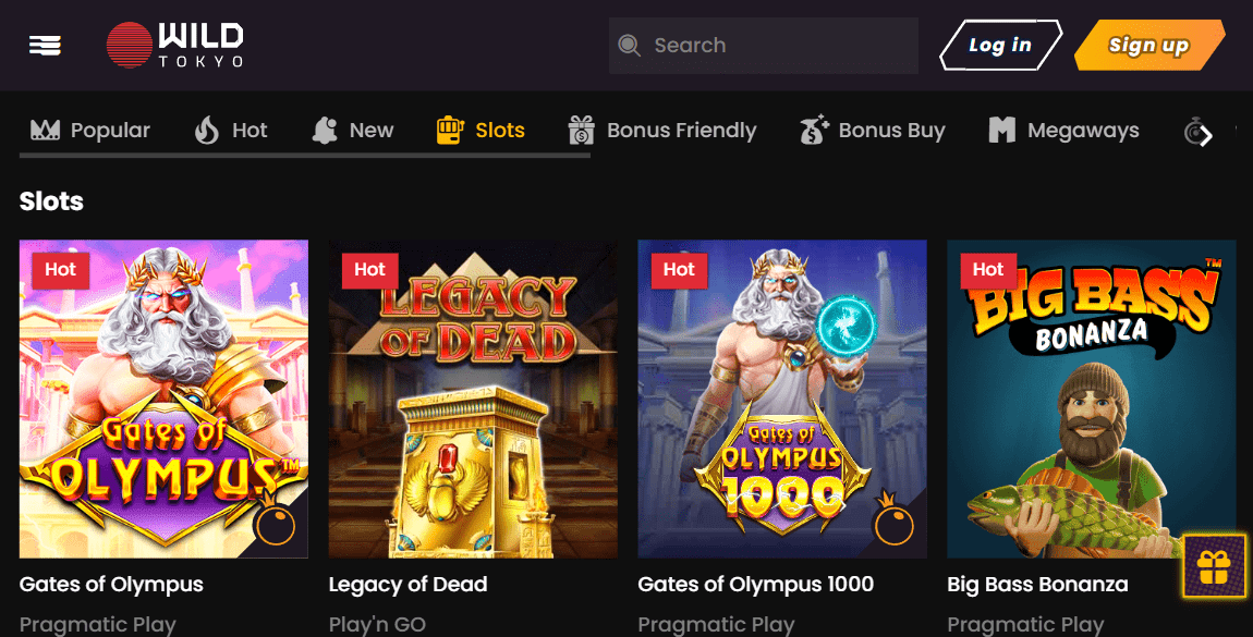
Wild Tokyo is a pokie’s fan paradise, at least it was for me, and I get very selective when it comes to pokies. There are nearly 6,000 games from top-rated providers, but if I had to recommend one, it would be Pragmatic Play’s Gates of Olympus 1000. This rendition of the popular original game with the same name boosts the gameplay with random multipliers, scatters, and free spins, among other features.
DragonSlots is no less impressive when it comes to pokies, boasting over 6,000 games sourced from more than 60 providers. Pokie diversity is ensured with high-, medium, and low-RTP games with different themes, of which Aztec Clusters was the best I played. If you want a game that promises frequent payouts, bonus rounds, and unconventional paylines in clusters, Aztec Clusters is a must-try.
King Billy Casino has Gold Rush With Johnny Cash, a game featuring the popular Hold and Win bonus game, alongside a bonus-buy feature, in-game jackpots, and a special Gold Respin feature. But this is one pokie in thousands, and is a small part of why King Billy ranks as a top real money casino online for pokies. The weekly bonuses, pokie tournaments, and loyalty prizes earned through playing pokies all contribute to the experience.
Top AU Casino Bonuses
| Casino | Top Bonus | Wagering Requirements | Validity |
|---|---|---|---|
| Richard Casino | 3% weekly cashback | 5x | 3 days |
| Neospin | 100 FS every Wednesday | 30x | N/A |
| DivaSpin | Up to A$1,050 + 50 FS on weekends | 35x | 10 days |

If you’re looking for a casino that offers a consistent stream of fair bonuses, Richard Casino is a fantastic choice, especially with its 3% weekly cashback. It’s a wonderful deal for both casual players and high-rollers, offering up to A$7,500. Plus, Richard Casino has many other exciting bonuses for you to explore, including regular promotions, weekly cash reloads, and free spin deals.
Neospin also offers a highly varied bonus menu, including 20% cashback, loyalty rewards, and up to A$1,000 on weekends. My favourite part is the 100 free spins available every Wednesday, a consistent feature of the Neospin bonus program. A key advantage of these free spins is that each one allows a bet value of up to A$10, exceeding the typical maximum bet of A$7.5 to A$8 found at other operators.
Weekends are my time to relax and enjoy my favourite casino games. At DivaSpin, I took advantage of their weekend bonus, claiming up to A$1,050 and 50 free spins with a A$100 deposit (minimum A$75). Other great promotions include a 25% live cashback for live dealer enthusiasts and 50 weekly free spins for pokie lovers.
Best Crypto Casinos for Aussies
| Casino | Crypto Bonus | Accepted Coins |
|---|---|---|
| Slots Gallery | Up to 1 BTC every day | Bitcoin, Dogecoin, Ethereum, Litecoin, Ripple, Tron, Tether |
| King Billy | 100% up to 0.5 BTC welcome bonus | Bitcoin, Ethereum, Litecoin, Tether |
| Slotozen | 100% up to A$1,000 + 100 FS | Bitcoin, Ethereum, Litecoin, Tether |
The three casinos you see in the table are ideal for going full crypto.
Slots Gallery, for instance, is fully equipped to accommodate crypto players with a huge bonus of up to 1 BTC every day and an extended selection of usable virtual currencies. Considering the price difference per cryptocurrency, the transfer limits vary for each coin, as shown in the cashier.
At King Billy, there is an exclusive crypto welcome bonus matching 100% of your crypto deposit up to 0.5 BTC, but I got a smaller amount, considering I was able to deposit in mBTC, and I didn’t really have a budget even remotely close to 0.5 BTC. King Billy supports other currencies as well (Litecoin, USDT), for which the regular bonuses may qualify, but you’d still have to contact customer service to make sure this is possible.
Finally, Slotozen is another excellent online Australian casino supporting crypto. Only about a handful of the most popular currencies are available (BTC, ETH, LTC, USDT), but you can use any available currency for bonuses so long as you satisfy the minimum qualifying deposit. The first deposit bonus of the welcome package provides plenty of bonus funds, 100% of your crypto deposit up to A$1,000, or currency equivalent.
What to Expect From the Top Online Casinos for Aussies
When you hear the word ‘casino’, you immediately think of pokies, blackjack, poker, and tournaments. And rightly so. The best real money online casinos in Australia go beyond the traditional casino experience, but you have to know what to look for. Let’s get started.
Game Options
- Highest RTP pokie: Gemhalla (97.17%) at Slots Gallery Casino
- Top jackpot game: Golden Dragon Inferno: Hold and Win at Neospin Casino
- Best game for high rollers: VIP Blackjack at PlayMojo Casino
Games bring a special appeal to every online casino. Our carefully ranked list of the best online Australian casinos showcases an exciting variety of games for everyone. Depending on the casino, you can find anywhere from 4,000 to over 15,000 games available. This selection includes classics like blackjack, roulette, baccarat, and poker in both automated and live versions.
The game volume at each casino continues to grow, thanks to the exclusive deals Aussie casino sites have with top-notch providers, such as Novomatic, BGaming, and Yggdrasil Gaming, which license incredible games.
Although they make up a smaller part of the game collections, instant win games (Plinko, Aviator) and game shows (Crazy Time, Dream Catcher, Mega Wheel) deserve an honourable mention.
Bonuses and VIP Offers
- Wagering requirements: 30x – 45x
- Min. required deposit: A$20 – A$45
- Validity period: 7 – 30 days
Bonuses and promotions enhance your gaming sessions. I’ve used various bonuses, including welcome bonuses, high-roller deals, cashback, free spins, and Fortune Wheel bonuses.
The welcome package is a cornerstone of all online casinos. Some offer standard and high-roller bonuses as matched deposit bonuses, giving a 100% match or more on one or multiple deposits. Matched deposit bonuses appear as regular promotions, usually between 50% and 70%. Free spins are available on select weekdays or weekends.
➡️ A few of the leading online casino sites in Australia, like DragonSlots and Neospin, provide exclusive promotions. These can be in the form of an ‘unlimited bonus’ or a Fortune Wheel bonus, like at DragonSlots, or a mystery bonus, like the one I found on All Star.
Payment Methods
- Max. deposit limits: A$4,000 – A$7,500
- Max. withdrawal limits: A$4,000 – A$88,000
- Payout time: 0 – 72 hours
When it comes to banking, there are a few essential things to consider: the available payment methods, payout speed, and transfer limits. Let’s quickly break them down.
The payment method you choose will be your channel for transferring money to and from an online casino in Australia for real money when you open an account. Many Aussie casinos accept e-vouchers like Neosurf or CashtoCode, but these are good only for deposits. In my experience, it’s best to choose a payment method like Visa, MasterCard, or MiFinity. These options can handle both deposits and withdrawals.
Cryptocurrencies offer a favourable option for deposits and withdrawals. Crypto transactions using Bitcoin, USDT, Ethereum, or Bitcoin Cash are the fastest payment methods and often have extended limits. For example, while maximum fiat deposits average A$6,000, some casinos, like OnLuck, impose no maximum on crypto deposits.
Withdrawals generally take anywhere from a couple of hours to up to 3 days, depending on the payment method. Crypto withdrawals usually process within minutes, while supported e-wallets are similar. Visa and MasterCard withdrawals can take 3 days, and bank transfers may take up to 5 or even 7 days in some instances.
Customer Support
Customer support is critical for new players and a vital resource for a positive experience as you play. I measure support based on the available means for contacting an online casino in Australia, the response time, and the provision of alternative support resources, such as a frequently asked questions page (FAQs).
Email support and live chat are the usual means of directly contacting your casino’s support desk. Our testers pay attention to the response time. Live chat assistants should not take more than a few minutes to respond to your questions. Some casinos have automated chatbots, in which case the response time is instant.
Emails take a bit longer to address, usually between 24 and 48 hours. Verified players, or those with a VIP status, often receive priority support and will hear back from the casino, usually within several hours. If you don’t want to wait for basic queries, you can open the FAQs page and browse through the answered questions.
Safety
Casino security is crucial if you play long-term. No one wants to spend their hard-earned cash on suspicious casino sites or gambling operators that cannot guarantee a basic level of security. I ensure the casino has basic security, such as a valid SSL or TLS encryption certificate. This is the first line of defence and ensures that all data exchanged between you and the casino has layered encryption protection.
An anti-fraud policy is also necessary, and this is a requirement for all licensed real-money online casinos in Australia. Anti-fraud measures are there to protect the casino and your account from malpractice and fraudulent behaviour.
Speaking of account protection, account security is a key part of overall casino security. Identity verification, know your customer (KYC) checks, and withdrawal verification are annoying but serve a valuable purpose for overall security.
Our Testing Criteria
Selecting the top online casinos for Aussies takes time, effort, and dedication. The whole team laboured over a period of about 3 months to test dozens of online casinos by reviewing essential benchmarks, including:
Safety and Licensing: As we just noted, security comes in many forms: data privacy, protection of funds, account security, and fraud prevention. If a casino is licensed, these aspects of security are almost always covered, which is why we only look for the best licensed casinos.
Game Variety: We prefer casinos with a rich game collection. Game variety in pokies, based on RTP, volatility, and features, matters. Table and card games, including live dealers, should offer options for every budget, from low-limit games to high-stakes tables.
Bonus Fairness: Bonuses should have manageable requirements that even low-stakes players can meet within the allotted period. Unless it’s an exclusive deal for high-rollers, casino bonuses must provide acceptable terms of use, such as wagering requirements and validity periods.
Mobile Experience: Each top online casino in Australia that makes our final list is fine-tuned for gambling on the go. We conduct tests on iOS and Android-powered devices and rank each casino’s performance.
Customer Support: It doesn’t matter if this is your first or 100th day at the casino; eventually, you will need help or assistance. We select casinos that provide professional support to all users and address queries and complaints in a timely and fair manner.
Payment Speed: We pick casinos where deposits are instant or up to a few minutes at most, and where payouts arrive in no more than 48 hours using card payments, e-wallets, and cryptocurrencies.
Fairness & RTP Audits: Games must be licensed from trusted game developers like Betsoft, Playson, NetGame, or Pragmatic Play. These, and other legitimate developers, run different audits to test a game’s return to player (RTP), mechanics, features, hit frequency, and ability to provide random results.
Player Reviews & Reputation: Analysing player comments on review sites is tricky, as unsatisfied users often leave baseless complaints. We verify all complaints for accuracy and cross-check positive comments to assess the casino’s true reputation.
Take a Look at Our Test Stats
| Total Casinos Tested | 150+ |
| Hours Spent | 600+ |
| Money Deposited | A$10,000 |
| Money Withdrawn | A$13,400 |
| Number of Withdrawals | 72 |
| Games Played | 250+ |
| Bonuses Claimed | 90+ |
| Chosen Casinos | 15 |
| Blacklisted Casinos | 21 |
The Good & Bad of Australian Online Casino Sites
We can’t say that the top online casinos in Australia are flawless, but the good thing is that the benefits far outweigh the negatives, which can be boiled down to a few minor flaws and deficits.
Playing your favourite casino games has never been easier, thanks to online casinos’ mobile compatibility with systems like Android and iOS. The best online casinos can be accessed via a browser or by installing a PWA on your
Maybe you want to dedicate time to a single, so a free spins bonus would fit the bill. Or, you want to explore table games and pokies, in which case a matched deposit bonus will be perfect. The better the bonus variety, the more options you have to pick one based on your gaming preferences.
Many of the real money online casinos on our list have a loyalty system. As you play, you earn loyalty points and can later convert your points for cash bonuses, free spins, or other available benefits.
Exclusive VIP perks are a step up from loyalty benefits. VIP membership is reserved for the top players and comes with advantages like priority payouts, personal account management, extended transaction limits, cashback, lowered bonus wagering, and exclusive bonuses.
When you’ve had enough, you want to cash out as fast as possible. Fast payouts through crypto, e-wallets, and even cards are a priority benchmark in our review process and one of the main advantages of Australian online casinos.
Bonus wagering can be a real pain to complete unless you enjoy grinding through the games. Some bonuses that have a wagering of over 40x can be challenging if you are not up to the task.
Most Aussie gambling sites lack a native app. While the best real money online casinos in Australia provide full mobile optimisation through mobile web browsers (PWAs), native apps offer a better experience and usually have extra features.
Poker is one of the all-time favourite casino games, but even the top online casinos have a shortage of live Caribbean, Omaha, or Hold’em poker tables.
Your Beginner's Guide to Australian Online Casinos
If you’re a beginner, it’s normal to have questions about which games to play, what RTP is, or which bonuses you can redeem. This part of our guide will help you quickly get on board with the basics of online gambling in Australia.
Best Games to Play
🎰 A top Australian online casino should offer high-RTP games (96% or over). Avoid pokies with RTP under 96% for long-term play. Choose high volatility pokies with features like free spins, respins, or bonus buy options, which can help trigger bigger wins. Also, unless playing casually, steer clear of 3-reel classic pokies as they often have simplified mechanics, low volatility, and lack special features.
🃏 Random number generator (RNG) and live dealer roulette provide different experiences. If you’re refining your strategy, start with low-stakes RNG table games before joining a live roulette or blackjack table. Look for games with low betting limits and a low house edge for basic bets.
⚡Instant games like Aviator or Plinko will keep you on the edge of your seat and can be a source of big and fast wins, but be cautious. These are risky games, and big losses can come hand in hand with big wins if you’re not careful.
What is RTP
RTP is a game’s house edge, i.e., a commercial advantage a game like pokie or roulette has over extended gambling periods. For example, a pokie game with 96.7% RTP has a 3.3% house edge. In other words, if you wager A$100, the game will, theoretically, return A$96.7. But RTP is not an exact measure, so you shouldn’t expect to receive the RTP-relevant amount for every A$100 you wager.
Bonuses to Avoid
If you’re eyeing casino bonuses, don’t rush. It’s important to match the terms with your gambling style. If you’re into pokies, free spins come with lower playthroughs than deposit matches; however, the max bet size may be significantly lower than the deposit bonus. On the other hand, 5% cashback with 2x playthrough is far better than 15% cashback with 20x wagering requirements. We’d also advise you to stay away from bonuses that expire in 24 or 48 hours – these WR will be impossible to clear, unless it’s just 2-3x.
Wagering Requirements Decoded
If the term ‘wagering requirements’ confuses you, it is the number of times you need to wager the bonus (and in some cases the deposit amount) and winnings from free spins. For example, a deposit bonus with 30x wagering means you must wager the bonus amount 30 times. For free spins, 30x wagering requirements apply to winnings. For example, if you win A$70 with your bonus spins, you must wager A$70*30 to be able to request a withdrawal.
Recommended Payment Options
The best Australian online casinos support various payment methods. But some are better than others, faster, or allow wider transfer limits. First, visit the casino’s cashier and see the transfer limits. Next, see if no fees are attached to payments like Visa, MasterCard, MiFinity, or cryptocurrencies.
⚠️ Check the average payout speed, and now you can make your choice. The ideal payment method should allow suitable transfer limits, no internal fees, and fast payouts. These features are common for crypto payments (Bitcoin, USDT, Litecoin, Ethereum), which ensure instant deposits, same-day withdrawals, no fees, and complete privacy and security. E-wallets like MiFinity can also be a suitable option for managing transactions to and from your casino account.
Legal Landscape: Can You Play at Online Casinos in Australia?
The short answer: yes. You can play at any Australian online casino for real money on our ranked list and cash out winnings. The legal landscape in Australia does not allow state-licensed casinos to operate in the country. So, online gambling companies have turned to international licensors like the Curacao Gaming Control Board to get certified.
The bottom line is, while online gambling in Australia is kept in check, overseas casinos accept legal-age Aussies and provide licensed gambling services. As a player, you can legally join any licensed casino if you are 18 or older.
Responsible Gambling – Tools for Staying in Control
Gambling shouldn’t and mustn’t be done under extreme emotions or without forethought. Here are some tips to guide you through your sessions:
- Make a budget: Decide how long and how much you can afford to spend (bet) and, based on that, create your gambling budget.
- Avoid large bets: There’s no point in risking much money on a single bet. Instead, set your bet value and stick to it.
- Apply limits: We recommend setting and adhering to personal spending limits by utilising the casino’s wager, deposit, and loss limits.
- Avoid credit cards: Credit card deposits can lead to negative balances, so it’s best to create a budget and store your funds using available debit cards, e-wallets, or crypto wallets.
- Know when to stop: Don’t gamble out of habit or routine. Try to have fun with every session. If you notice a lack of interest, it’s time to take a break.
Final Verdict: What’s the Best Online Casino in Australia?
The best online casino in Australia is any vetted gambling site that meets your personal preferences. Think deposit limits, accepted payment methods, bonus terms, available games, and mobile compatibility.
Based on our review methodology and the above-listed parameters, the best casino in Australia is Stay Casino.
But don’t let this stop you from doing some research on your own. Our ranked list includes 15 of the best real money online casinos in Australia, and we broke down the top sites based on aspects like mobile gambling, best for crypto, or top sites for pokies.
Who is GISCafe.com?
Ewan McAllister
Ewan McAllister is the main author at GISCafe and a seasoned online gambling expert with years of hands-on industry experience.
Before stepping into writing and casino analysis, he worked as a croupier and later as a casino manager, gaining a deep understanding of the inner workings of both land-based and online gambling. His expertise spans across all areas of casino gaming, from testing pokies and evaluating online casinos to mastering blackjack strategy and understanding player behavior.
At GISCafe, Ewan combines his practical background with sharp analytical skills to deliver honest, well-researched insights that help readers make informed decisions. Known for his straightforward approach and passion for fairness in gambling, he has become a trusted voice in the industry.
Away from the tables and spreadsheets, Ewan is also a die-hard Arsenal fan, never missing a chance to support his club.
FAQ
StayCasino is the best real money online casino in Australia. It offers over 400 live casino games, more than 4,000 pokies, a PWA app, and weekly and welcome bonuses.
The minimum deposit range to play at Australian casino sites is typically between A$20 and A$40.
Every listed online Australian casino provides cash deposit bonuses and free spins usable on select pokies.
Withdrawal processing depends on the casino and payment method used, but is usually between 24 and 72 hours, or under 24 hours using cryptocurrencies.
Yes, Australian online gambling sites either offer progressive jackpots on some or most games, or have a special section for jackpot games with progressive or fixed jackpots.